In our increasingly digital world powered by software and web-based applications, Machine Learning (ML) applications have become extremely popular. The ML community uses several Deep Learning (DL) frameworks like Tensorflow*, PyTorch*, and Keras* to solve real world problems.

However, understanding computational and memory bottlenecks in DL code like Python or C++ is challenging and often requires significant effort due to the presence of hierarchical layers and non-linear functions. Frameworks like Tensorflow* and PyTorch* provide native tools and APIs that enable the collection and analysis of performance metrics during different stages of Deep Learning Model development. But the scope of these profiling APIs and tools is quite limited. They do not provide deep insight at the hardware level to help you optimize different operators and functions in the Deep Learning models.

In this recipe, learn how you can use VTune Profiler to profile a Python workload and improve data collection with additional APIs.

This recipe uses the Intel® Distribution for Python and Data Parallel Extensions for Python.

Content Expert: Rupak Roy, Lalith Sharan Bandaru, Rob Albrecht-Mueller,

• INGREDIENTS

• DIRECTIONS:

  1. Install and Set Up Python Package.
  2. Profile NumPy Implementation of Pairwise Distance with Hotspots Analysis.
  3. Profile Data Parallel Extension for NumPy Implementation of Pairwise Distance with Hotspots Analysis.
  4. Profile Data Parallel Extension for Numba Implementation of Pairwise Distance with Hotspots Analysis.

Ingredients

Here are the hardware and software tools you need for this recipe.

• Application: This recipe uses the NumPy example of an algorithm for pairwise distance calculation. The NumPy example has three implementations, which use the following packages:

  • Intel Distribution for Python NumPy
  • Data Parallel Extension for NumPy
  • Data Parallel Extension for Numba on GPU

  Here is a code snippet from the NumPy example:

  import numpy as np
  import time
  
  #compute pairwise distance
  def pairwise_distance(data, distance):
      data_sqr = np.sum(np.square(data), dtype = np.float32, axis=1)
      np.dot(data, data.T, distance)
      distance *= -2
      np.add(distance, data_sqr.reshape(data_sqr.size, 1), distance)
      np.add(distance, data_sqr, distance)
      np.sqrt(distance, distance)
  
  data = np.random.ranf((10*1024,3)).astype(np.float32)
  distance = np.empty(shape=(data.shape[0], data.shape[0]), dtype=np.float32)
  
  
  #time pairwise distance calculations
  start = time.time()
  pairwise_distance(data, distance)
  print("Time to Compute Pairwise Distance with Stock NumPy on CPU:", time.time() - start)
  

• Analysis Tool: User-mode sampling and tracing collection with VTune Profiler (version 2022 or newer)

• Compiler: Intel® oneAPI DPC++/C++ Compiler

• Software: Intel® Distribution for Python* and Data Parallel Extensions for Python

• Software Components:

  • dpcpp-llvm-spirv 2024.1.0
  • dpctl 0.16.0
  • dpnp 0.14.0+189.gfcddad2474
  • mkl-fft 1.3.8
  • mkl-random 1.2.4
  • mkl-service 2.4.0
  • mkl-umath 0.1.1
  • numba 0.59.0
  • numba-dpex 0.21.4
  • numpy 1.26.4
  • packaging 23.1
  • ittapi 1.1.0
  • setuptools 67.7.2
  • TBB 0.2

• CPU: Intel® Xeon® Platinum 8480+

• GPU: Intel® Data Center GPU Max 1550

• Operating System: Linux*, Ubuntu Server 22.04.3 LTS

Install and Set Up the Python Package

1. Install Intel Distribution for Python.
2. Create a virtual environment for Intel Distribution for Python.

   python -m venv pyenv 
   source ./pyenv/bin/activate
   

3. Install the Python packages.

   pip install numpy==1.26.4
   pip install dpnp
   pip install numba
   pip install numba-dpex
   pip install ittapi
   

Profile NumPy Implementation of Pairwise Distance with Hotspots Analysis

Insert Intel® Instrumentation and Tracing Technology (ITT) APIs in the NumPy implementation to designate logical tasks.

import numpy as np
import ittapi

def pairwise_distance(data, distance):
    with ittapi.task('pairwise_sum'):
        data_sqr = np.sum(np.square(data), dtype = np.float32, axis=1)
    with ittapi.task('pairwise_dot'):
        np.dot(data, data.T, distance)
    distance *= -2
    with ittapi.task('pairwise_add'):
        np.add(distance, data_sqr.reshape(data_sqr.size, 1), distance)
        np.add(distance, data_sqr, distance)
    with ittapi.task('pairwise_sqrt'):
        np.sqrt(distance, distance)

with ittapi.task('data_load'):
    data = np.random.ranf((100*1024,3)).astype(np.float32)
    distance = np.empty(shape=(data.shape[0], data.shape[0]), dtype=np.float32)

Next, run a Hotspots analysis on the annotated NumPy code. This analysis is a good starting point to identify the most time-consuming regions in the code. Make sure to enable user-mode sampling in the analysis so that you can see profiling information about the Python code.

In the command line, type:

vtune -collect hotspots -knob sampling-mode=sw --python3 NumPy-Implementation.py

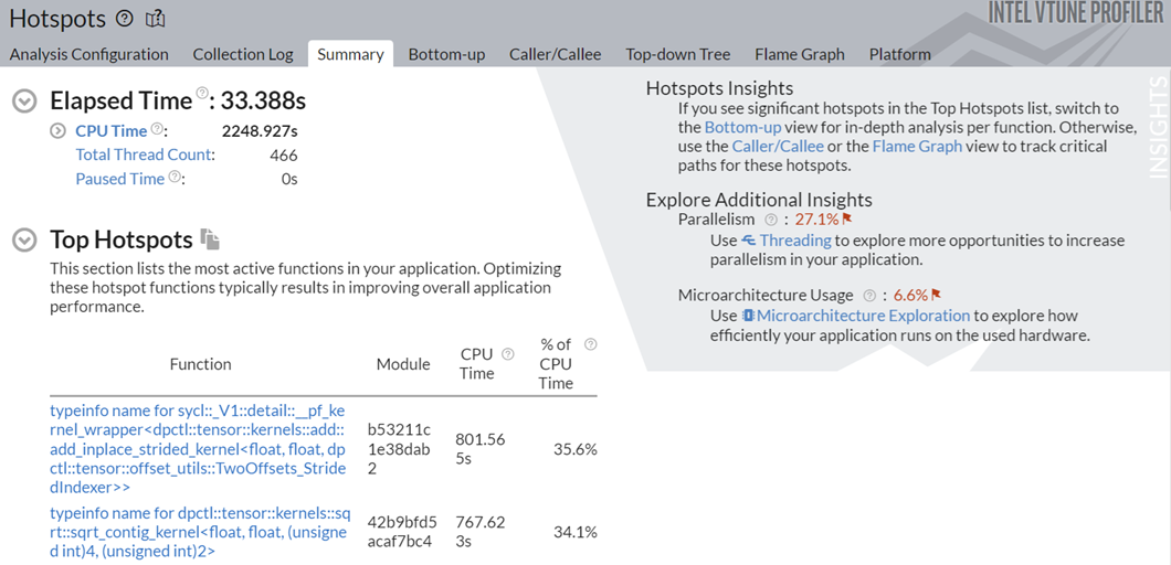
This command runs the Hotspots analysis in sampling mode on the NumPy implementation. Once the analysis is completed, profiling results display in the Summary window.

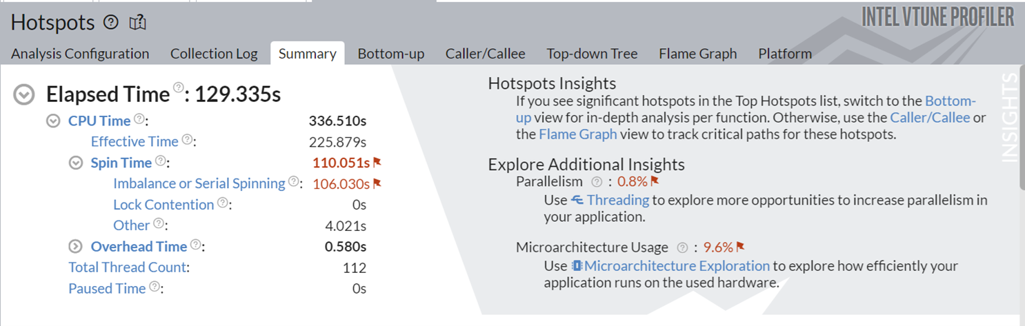
This implementation took around 130s to execute, and also spending significant time on serial spinning. The Additional Insights section in the top right corner informs you to consider running Threading and Microarchitecture Exploration analyses to understand these bottlenecks better.

Next, let us look at the top tasks in the application:

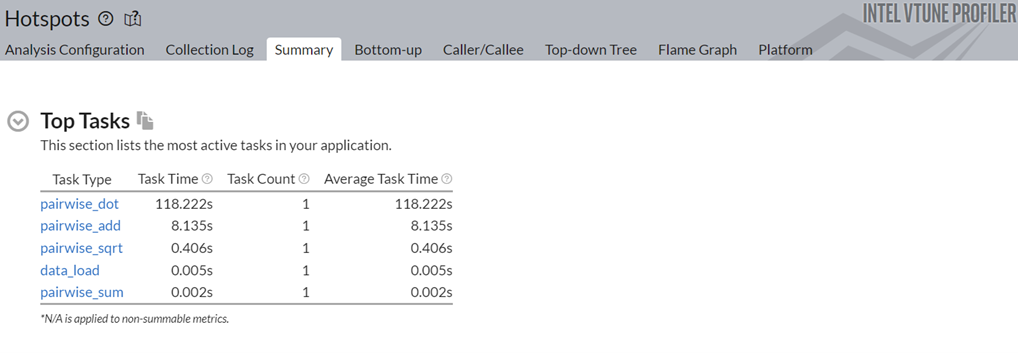
Click on the top task in the table, the pairwise_dot task. Switch to the Bottom-up view to examine the APIs inside this task.

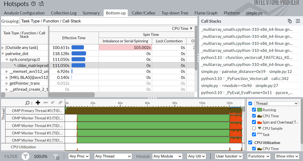
In the figure above, in the Task Type column, the pairwise_dot task has several APIs associated with it. The syrk oneMKL routine is the most time-consuming routine, followed by memset and other operations.

Switch to the simple.py source code window. Here, you see that the np.dot function is responsible for 33% of the total execution time.

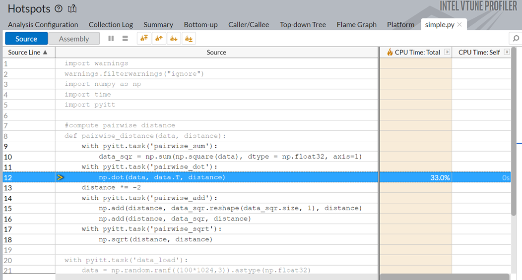
Optimizing the np.dot function or replacing it with a better API could significantly improve the runtime of the application.

Profile Data Parallel Extension for NumPy Implementation of Pairwise Distance with Hotspots Analysis

Try to optimize the bottlenecks identified in the previous step. Switch from the NumPy implementation to the Data Parallel Extension for NumPy Implementation. To make this switch, replace numpy with dpnp in the original code, as shown below:

import dpnp as np
import time

#compute pairwise distance
def pairwise_distance(data, distance):
    data_sqr = np.sum(np.square(data), dtype = np.float32, axis=1)
    np.dot(data, data.T, distance)
    distance *= -2
    np.add(distance, data_sqr.reshape(data_sqr.size, 1), distance)
    np.add(distance, data_sqr, distance)
    np.sqrt(distance, distance)

data = np.random.ranf((10*1024,3)).astype(np.float32)
distance = np.empty(shape=(data.shape[0], data.shape[0]), dtype=np.float32)


#time pairwise distance calculations
start = time.time()
pairwise_distance(data, distance)
print("Time to Compute Pairwise Distance with Stock NumPy on CPU:", time.time() - start)

Repeat the Hotspots analysis on the Data Parallel Extension for NumPy Implementation.

When the profiling is complete, open results in the Summary window.

Observe a significant improvement in the total runtime from 130s to 33.38s.

To understand the reasons behind this improvement, go to the Top Tasks section in the Summary window.

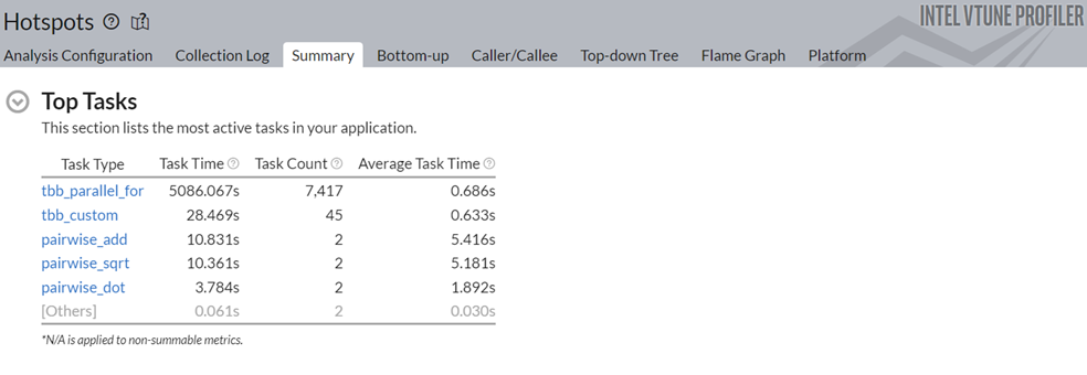
Notice that the task time for the pairwise_dot task dropped from 118.2s to 3.78s. To learn about the changes introduced by the Data Parallel Extension for NumPy Implementation, switch to the Bottom-up window.

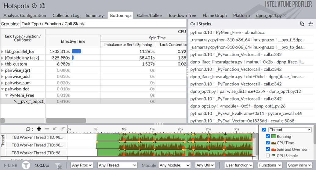
You see that the pairwise_dot function now uses dpctl APIs, unlike the NumPy implementation that used the oneMKL API previously. The dpctl APIs contribute to the performance boost.

Going by the recommendation in the Additional Insights section of the Summary pane, try to increase parallelism for this application. To do so, use the Numba implementation next.

Profile Data Parallel Extension for Numba Implementation of Pairwise Distance with Hotspots Analysis.

Use this code for the Numba implementation of pairwise distance:

from numba_dpex import dpjit
from numba import prange
@dpjit #using Numba JIT compiler optimizations, now on any SYCL device
def pairwise_distance(data, distance):
    float0 = data.dtype.type(0)

    #prange used for parallel loops for further opt
    for i in prange(data.shape[0]):
        for j in range(data.shape[0]):
            d = float0
            for k in range(data.shape[1]):
                d += (data[i, k] - data[j, k])**2

            distance[j, i] = np.sqrt(d)

data = np.random.ranf((10*1024,3)).astype(np.float32)
distance = np.empty(shape=(data.shape[0], data.shape[0]), dtype=np.float32)

#do compilation first run, wecode- will calculate performance on subsequent runs
#wrapper consistent with previous np and dpnp scripts
pairwise_distance(data, distance)

#time pairwise distance calculations
start = time.time()
pairwise_distance(data, distance)
#using heterogeneous

Next, run the GPU Compute/Media Hotspots analysis on the Numba implementation.

vtune -collect gpu-hotspots –-python numba_implementation.py

When the analysis is completed, examine the results in the Summary window:

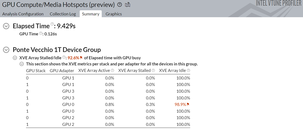
Notice a 3x speedup in performance when using the Numba implementation.

You also see that the Stack 0 of GPU 0 was the only stack that was used in the four GPUs available. Idle time was high and this is typical for small workloads. Yet, there was significant improvement in the total execution time.

Switch to the Graphics window. Group the results in the table here by Computing Task.

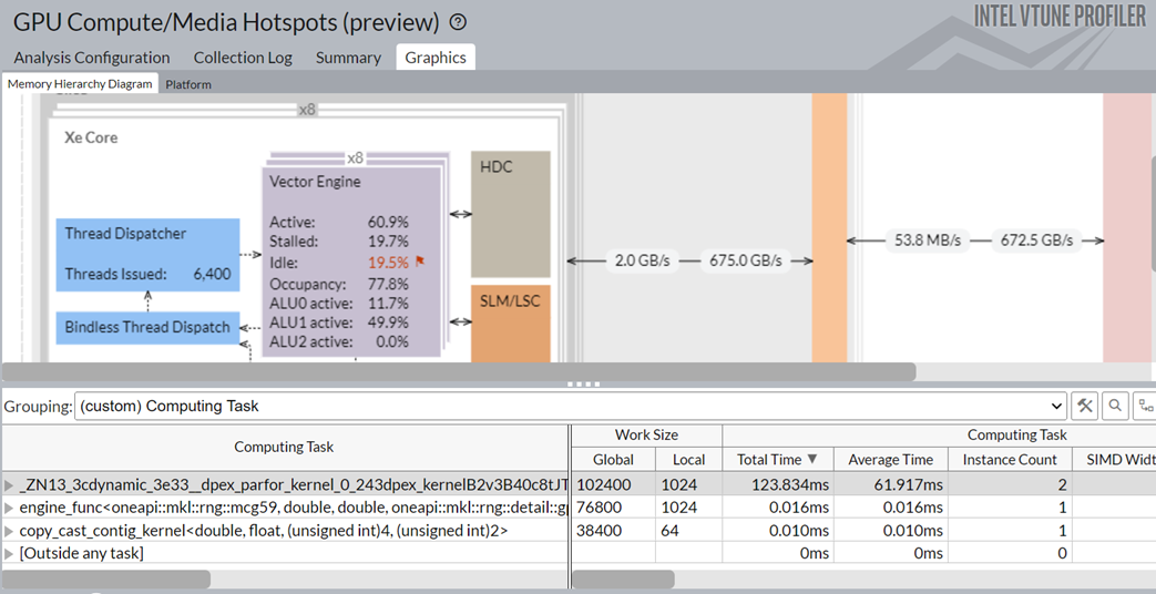
You see these details:

• The Numba dpex_kernel consumed the most time. This was expected.
• The Numba dpex_kernel kept the GPU vector engines busy. The activity level of the X^e Vector Engine was ~60.9%.

If you use a large workload with several kernels, use the computing-tasks-of-interest knob to specify kernels of interest.