Visible to Intel only — GUID: GUID-FE1BFE5D-3110-4AAB-91D4-D6143C454160
basic_statistics_dense_batch.cpp
basic_statistics_dense_online.cpp
column_accessor_homogen.cpp
cor_dense_batch.cpp
cor_dense_online.cpp
cov_dense_batch.cpp
cov_dense_biased_batch.cpp
cov_dense_biased_online.cpp
cov_dense_online.cpp
csr_accessor.cpp
csr_table.cpp
dbscan_brute_force_batch.cpp
df_cls_hist_batch.cpp
df_cls_hist_batch_random.cpp
df_cls_traverse_model.cpp
df_reg_hist_batch.cpp
df_reg_hist_batch_random.cpp
df_reg_traverse_model.cpp
heterogen_table.cpp
homogen_table.cpp
kmeans_init_dense.cpp
kmeans_lloyd_dense_batch.cpp
knn_cls_brute_force_dense_batch.cpp
knn_reg_brute_force_dense_batch.cpp
knn_search_brute_force_dense_batch.cpp
linear_kernel_dense_batch.cpp
linear_regression_dense_batch.cpp
linear_regression_dense_online.cpp
logistic_regression_dense_batch.cpp
pca_cor_dense_batch.cpp
pca_cor_dense_online.cpp
pca_cov_dense_batch.cpp
pca_cov_dense_online.cpp
pca_precomputed_cor_dense_batch.cpp
pca_precomputed_cov_dense_batch.cpp
pca_svd_dense_batch.cpp
rbf_kernel_dense_batch.cpp
read_batch.cpp
svm_two_class_thunder_dense_batch.cpp
basic_statistics_dense_batch.cpp
basic_statistics_dense_online.cpp
column_accessor_homogen.cpp
connected_components_batch.cpp
cor_dense_batch.cpp
cor_dense_online.cpp
cov_dense_batch.cpp
cov_dense_biased_batch.cpp
cov_dense_biased_online.cpp
cov_dense_online.cpp
csr_accessor.cpp
csr_table.cpp
dbscan_brute_force_batch.cpp
df_cls_dense_batch.cpp
df_reg_dense_batch.cpp
directed_graph.cpp
graph_service_functions.cpp
heterogen_table.cpp
homogen_table.cpp
jaccard_batch.cpp
jaccard_batch_app.cpp
kmeans_init_dense.cpp
kmeans_lloyd_dense_batch.cpp
knn_cls_brute_force_dense_batch.cpp
knn_cls_kd_tree_dense_batch.cpp
knn_search_brute_force_dense_batch.cpp
linear_kernel_dense_batch.cpp
linear_regression_dense_batch.cpp
linear_regression_dense_online.cpp
logloss_dense_batch.cpp
louvain_batch.cpp
pca_cor_dense_batch.cpp
pca_cor_dense_online.cpp
pca_cov_dense_batch.cpp
pca_cov_dense_online.cpp
pca_precomputed_dense_batch.cpp
pca_svd_dense_batch.cpp
pca_svd_dense_online.cpp
polynomial_kernel_dense_batch.cpp
rbf_kernel_dense_batch.cpp
read_batch.cpp
shortest_paths_batch.cpp
sigmoid_kernel_dense_batch.cpp
subgraph_isomorphism_batch.cpp
svm_multi_class_thunder_csr_batch.cpp
svm_multi_class_thunder_dense_batch.cpp
svm_nu_cls_thunder_csr_batch.cpp
svm_nu_cls_thunder_dense_batch.cpp
svm_nu_reg_thunder_csr_batch.cpp
svm_nu_reg_thunder_dense_batch.cpp
svm_reg_thunder_csr_batch.cpp
svm_reg_thunder_dense_batch.cpp
svm_two_class_smo_csr_batch.cpp
svm_two_class_smo_dense_batch.cpp
svm_two_class_thunder_csr_batch.cpp
svm_two_class_thunder_dense_batch.cpp
triangle_counting_batch.cpp
K-Means Clustering
Density-Based Spatial Clustering of Applications with Noise
Correlation and Variance-Covariance Matrices
Principal Component Analysis
Principal Components Analysis Transform
Singular Value Decomposition
Association Rules
Kernel Functions
Expectation-Maximization
Cholesky Decomposition
QR Decomposition
Outlier Detection
Distance Matrix
Distributions
Engines
Moments of Low Order
Quantile
Quality Metrics
Sorting
Normalization
Optimization Solvers
Decision Forest
Decision Trees
Gradient Boosted Trees
Stump
Linear and Ridge Regressions
LASSO and Elastic Net Regressions
k-Nearest Neighbors (kNN) Classifier
Implicit Alternating Least Squares
Logistic Regression
Naïve Bayes Classifier
Support Vector Machine Classifier
Multi-class Classifier
Boosting
Visible to Intel only — GUID: GUID-FE1BFE5D-3110-4AAB-91D4-D6143C454160
Decision Forest Classification and Regression (DF)
Decision Forest (DF) classification and regression algorithms are based on an ensemble of tree-structured classifiers, which are known as decision trees. Decision forest is built using the general technique of bagging, a bootstrap aggregation, and a random choice of features. For more details, see [Breiman84] and [Breiman2001].
Operation |
Computational methods |
Programming Interface |
|||
Mathematical formulation
Training
Given n feature vectors  of size p, their non-negative observation weights
  and n responses
  ,
,
Classification
 , where C is the number of classes
Regression

the problem is to build a decision forest classification or regression model.
The library uses the following algorithmic framework for the training stage. Let  be the set of observations. Given positive integer parameters, such as the number of trees B, the bootstrap parameter
  , where f is a fraction of observations used for a training of each tree in the forest, and the number of features per node m, the algorithm does the following for
  :
:
Selects randomly with replacement the set
 of N vectors from the set S. The set is called a bootstrap set.
Trains a decision tree classifier
 on using parameter m for each tree.
Decision treeT is trained using the training set D of size N. Each node t in the tree corresponds to the subset  of the training set D, with the root node being D itself. Each internal node t represents a binary test (split) that divides the subset
  in two subsets,
  and
and  , corresponding to their children,
  and
and  .
.
Training method: Dense
In the dense training method, all possible data points for each feature are considered as possible splits for the current node and evaluated best-split computation.
Training method: Hist
In the hist training method, only bins are considered for best split computation. Bins are continuous intervals of data points for a selected feature. They are computed for each feature during the initialization stage of the algorithm. Each value from the initially provided data is substituted with the value of the corresponding bin. It decreases the computational time complexity from  to
to  , but decreases algorithm accuracy, where
  is number of rows,
  is number of bins, and
  is number of selected features.
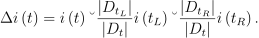
Split strategy
NOTE:
The random split strategy is supported only for the hist method. The dense method supports only the best strategy.
There are two split strategies for building trees:
Best splitter
The threshold for a node is chosen as the best among all bins and all selected features according to split criteria(see Split Criteria below). The computational time complexity for the best splitter is  for each node. The best splitting strategy builds a tree with optimal splits on each level.
Random splitter
The threshold for a node is chosen randomly for each selected feature. The split threshold is chosen as the best among all pairs (feature, random threshold) according to split criteria(see Split Criteria below). The computational time complexity for the random splitter as  for each node. The random splitting strategy does not build a tree with optimal trees, but in the case of big tree ensembles, it provides a more robust model comparing to the best strategy.
Split Criteria
The metric for measuring the best split is called impurity, i(t). It generally reflects the homogeneity of responses within the subset in the node t.
Classification
Gini index is an impurity metric for classification, calculated as follows:
where
D is a set of observations that reach the node;
 is specified in the table below:
Without sample weights |
With sample weights |
|---|---|
|
|
Regression
MSE is an impurity metric for regression, calculated as follows:
Without sample weights |
With sample weights |
|---|---|
|
|
|
|


 , which is equivalent to the number of elements in S
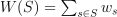
Let the impurity decrease in the node t be
Termination Criteria
The library supports the following termination criteria of decision forest training:
- Minimal number of observations in a leaf node
-
Node t is not processed if
 is smaller than the predefined value. Splits that produce nodes with the number of observations smaller than that value are not allowed.
 - Minimal number of observations in a split node
-
Node t is not processed if
is smaller than the predefined value. Splits that produce nodes with the number of observations smaller than that value are not allowed. - Minimum weighted fraction of the sum total of weights of all the input observations required to be at a leaf node
-
Node t is not processed if
is smaller than the predefined value. Splits that produce nodes with the number of observations smaller than that value are not allowed. - Maximal tree depth
-
Node t is not processed if its depth in the tree reached the predefined value.
- Impurity threshold
-
Node t is not processed if its impurity is smaller than the predefined threshold.
- Maximal number of leaf nodes
-
Grow trees with positive maximal number of leaf nodes in a best-first fashion. Best nodes are defined by relative reduction in impurity. If maximal number of leaf nodes equals zero, then this criterion does not limit the number of leaf nodes, and trees grow in a depth-first fashion.
Tree Building Strategies
Maximal number of leaf nodes defines the strategy of tree building: depth-first or best-first.
Depth-first Strategy
If maximal number of leaf nodes equals zero, a decision tree is built using depth-first strategy. In each terminal node t, the following recursive procedure is applied:
Stop if the termination criteria are met.
Choose randomly without replacement m feature indices
 .
.For each
 , find the best split
  that partitions subset and maximizes impurity decrease
  .
.A node is a split if this split induces a decrease of the impurity greater than or equal to the predefined value. Get the best split
 that maximizes impurity decrease
  in all splits.
Apply this procedure recursively to
and .
Best-first Strategy
If maximal number of leaf nodes is positive, a decision tree is built using best-first strategy. In each terminal node t, the following steps are applied:
Stop if the termination criteria are met.
Choose randomly without replacement m feature indices
.For each
, find the best split that partitions subset and maximizes impurity decrease .A node is a split if this split induces a decrease of the impurity greater than or equal to the predefined value and the number of split nodes is less or equal to
 . Get the best split that maximizes impurity decrease in all splits.
Put a node into a sorted array, where sort criterion is the improvement in impurity
 . The node with maximal improvement is the first in the array. For a leaf node, the improvement in impurity is zero.
Apply this procedure to
and and grow a tree one by one getting the first element from the array until the array is empty.
Inference
Given decision forest classification or regression model and vectors  , the problem is to calculate the responses for those vectors.
Inference methods: Dense and Hist
Dense and hist inference methods perform prediction in the same way. To solve the problem for each given query vector  , the algorithm does the following:
Classification
For each tree in the forest, it finds the leaf node that gives its label. The label y that the majority of trees in the forest vote for is chosen as the predicted label for the query vector .
Regression
For each tree in the forest, it finds the leaf node that gives the response as the mean of dependent variables. The mean of responses from all trees in the forest is the predicted response for the query vector .
Additional Characteristics Calculated by the Decision Forest
Decision forests can produce additional characteristics, such as an estimate of generalization error and an importance measure (relative decisive power) of each of p features (variables).
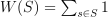
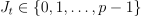
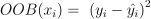
Out-of-bag Error
The estimate of the generalization error based on the training data can be obtained and calculated as follows:
Classification
For each vector
in the dataset X, predict its label  by having the majority of votes from the trees that contain in their OOB set, and vote for that label.
Calculate the OOB error of the decision forest T as the average of misclassifications:
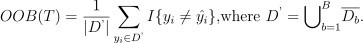
If OOB error value per each observation is required, then calculate the prediction error for
: 
Regression
For each vector
in the dataset X, predict its response as the mean of prediction from the trees that contain in their OOB set: , where
 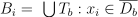 and
and  is the result of prediction by .
Calculate the OOB error of the decision forest T as the Mean-Square Error (MSE):
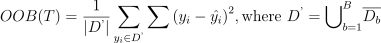
If OOB error value per each observation is required, then calculate the prediction error for
:
Variable Importance
There are two main types of variable importance measures:
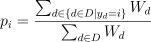
Mean Decrease Impurity importance (MDI)
Importance of the j-th variable for predicting Y is the sum of weighted impurity decreases
 for all nodes t that use
  , averaged over all B trees in the forest:
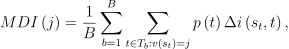
where
 is the fraction of observations reaching node t in the tree , and
  is the index of the variable used in split .
Mean Decrease Accuracy (MDA)
Importance of the j-th variable for predicting Y is the average increase in the OOB error over all trees in the forest when the values of the j-th variable are randomly permuted in the OOB set. For that reason, this latter measure is also known as permutation importance.
In more details, the library calculates MDA importance as follows:
Let
 be the set of feature vectors where the j-th variable is randomly permuted over all vectors in the set.
Let
 be the OOB error calculated for
  on its out-of-bag dataset
  .
.Let
 be the OOB error calculated for using
  , and its out-of-bag dataset is permuted on the j-th variable. Then
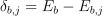 is the OOB error increase for the tree .
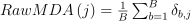 is MDA importance.
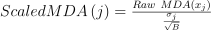 , where
  is the variance of
Programming Interface
Refer to API Reference: Decision Forest Classification and Regression.
Distributed mode
The algorithm supports distributed execution in SMPD mode (only on GPU).