
Overview
Financial markets rely on mathematical models and their application to very large datasets to analyze, predict, and assess the risk of many securities. Common examples include pricing derivative securities, such as options and risk management, especially portfolio management applications. In the next step, financial engineering combines the mathematical theory of quantitative finance with computational simulations to make price, trade, hedge, and other investment decisions. The cornerstones of these calculations are:
- Numerical solutions for differential equations
- Securities pricing simulations based on many randomly seeded Monte Carlo simulations
Many financial instruments, such as equities, equity indices, commodities, bonds, currencies, convertible debt contracts, and even derivatives (like swaps and futures) depend on and are influenced by the options market. This makes it critically important for financial markets to reliably model option pricing behavior so that their impact on other asset classes can be properly understood.
The Greek Risk Parameters
The Greeks are the basis for assessing risk profiles of options and other asset classes. They are a set of risk parameters associated with options. A Greek symbol is used to designate each of these risks. There is a long list of risks that are being tracked. The most common ones are:
- Theta: time decay or sensitivity of the option value to the passage of time
- Rho: sensitivity of an option's value to interest rate changes
- Delta: sensitivity of an option's value to changes in the underlying asset price
- Gamma: second-order option value sensitivity to the rate of change between an option's delta and the underlying asset's price
- Vega (nu): sensitivity of an option's value to underlying asset price volatility
The numerical solutions for the differential equations representing the Greeks heavily rely on various math functions, such as square roots, exponentials, logarithms, normal random number generation, correlated random number generation, path generation, and more.
Intel® oneAPI Math Kernel Library (oneMKL) has you covered for these calculations using C, Fortran, and SYCL* APIs. For open source, open standards-based implementations taking advantage of multiarchitecture GPU accelerator offload, the SYCL API in the Unified Acceleration Foundation (UXL Foundation*) open source oneAPI Math Library (oneMath) project can be used.
The very compute-intensive iterative process of combining a simulation and numerical solution of differential equations makes financial asset risk modeling an ideal candidate for highly parallel programming models like SYCL.
Let us take a closer look at the various prediction models for market valuation and how they benefit from running an optimized random number generator (RNG or RAND) on highly parallel compute engines like Intel® Data Center GPU Max Series or the integrated GPUs in the latest generation Intel® Core™ Ultra mobile processors.
Random Number Generation and Simulations in Finance
The most common simulation models in modern quantitative finance are:
- Binomial options pricing model (BOPM)
- Black-Scholes model (BSM)
- Heston model
- European Monte Carlo (EMC) options model
- American Monte Carlo (AMC) options model
Each model has its purpose:
Binomial Options Pricing Model (BOPM)
This model uses a generalizable numerical method for the valuation of options. The model uses a discrete-time (lattice-based) decision tree of the varying price over time. This approach is beneficial when an option can be exercised at any point in time, even before its maturity date. The investment risk needs to be calculated at any number of future time stamps. The BOPM is based on the description of an investment over time rather than a single point, making it popular for options traded on American stock markets.
Binomial options pricing is computationally slower than other alternatives, like Black-Scholes. In addition, BOPM does not work well with a higher number of market condition parameters. However, it is frequently used for options with simple dependencies, as it provides accurate results, especially over longer investment periods.
Black-Scholes Model (BSM)
Black-Scholes posits that stock shares or futures contracts have a log-normal distribution of prices following a random walk with constant drift and volatility. Based on this assumption, it is commonly regarded as the best model for pricing an options contract. The Black-Scholes equation requires six variables. These inputs are volatility, the underlying asset price, the option’s strike price, the time until the option's expiration, the risk-free interest rate, and the type of option (call or put). One caveat is that high-risk downward moves tend to happen more often in real-world markets than the BSM risk distribution predicts.
Heston Model
The Heston model addresses this shortcoming of BSM by describing the evolution of a financial asset's volatility over time. It assumes that asset valuation and volatility are neither constant nor deterministic but stochastic. The partial differential equation at the heart of the Heston model is calculated using a Monte Carlo simulation of many continuous random walks through its input parameters. The Heston model is a partial differential equation that cannot be solved exactly. Using it to price options requires mathematical approximation techniques. Applying this approach specifically to American and European options models leads us to the next discussion items.
European Monte Carlo (EMC) Options Model
Monte Carlo simulation is a widely used technique based on repeated random sampling to determine the properties of different investment strategy outcomes. For European options, pricing is a simple financial benchmark based on the assumption that we have a well-known fixed time until options exercise at maturity.
Let St represent the stock price at a given moment t that follows the stochastic process described by:
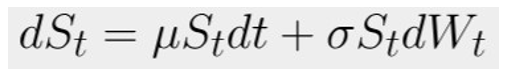
where μ is the drift and σ is the volatility (assumed to be constants), W = (Wt). t ≥ 0 represents the random sampling distribution. dt is a time step.
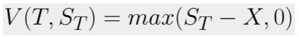
The value of a European option V(t,St) defined for 0 ≤ t ≤ T depends on the price St of the underlying stock. The option is issued at t = 0 and exercised at a time t = T called maturity. For European call and put options, the value of the option at maturity V(T,ST) is defined as:
A call option:
A put option:
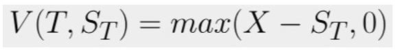
where X is the strike price. The problem is to estimate the value V(0,S0).
The Monte Carlo approach to this problem is a simulation of n possible realizations of ST, followed by averaging V(T,ST), and then discounting the average by factor e-rt to get the present value of option V(0,S0). ST follows a log-normal distribution:
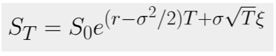
where ξ is a random variable of the standard normal distribution.
American Monte Carlo (AMC) Options Model
The AMC options model is a bit trickier as the exercise date for an option is not fixed. This option type can be exercised at any time at or before maturity. To accommodate this, a least squares Monte Carlo technique is employed. It follows an iterative two-step procedure:
- A backward induction process is performed, where a value is recursively assigned to every state at every timestep. The value is defined as the least squares regression against the market price of the option value at that time. The option value for this regression is defined as the value of exercise possibilities (dependent on market price) plus the value of the timestep value of a possible exercise.
- When all states are valued for every timestep, the value of the option is calculated by moving through the timesteps and states by making an optimal decision on an option exercise at every step on the hand of a price path, and the value of the state that it would result in. This second step can be done with multiple price paths to add a stochastic effect to the procedure.
The AMC options model adds another level of a parallel running path compute intensity to the problem.
Let us have a look at simplified reference sample benchmark implementations of these different methods to illustrate the benefit of oneMKL, SYCL APIs, and GPU offload for these compute-intensive tasks.
Implement and Benchmark Different Option Prediction Methods using oneMKL
The semantic difference between financial option models leads to differences in implementation.
Binomial, Black-Scholes, and EMC need initial data to be generated. For oneAPI samples, oneMKL random number generation is used to generate initial values of stock prices, strikes, and years for each option. The data is generated using a random uniform distribution. This part is not usually measured.
Figure 1. Using oneMKL for initial random number generation
The measuring part of binomial and Black-Scholes use only arithmetic operations and standard math functions like logarithm, square root, and exponent. So, the kernel of benchmarks has heavy computations that are easily parallelized as each SYCL work item processes one option (binomial) or a portion of options (Black-Scholes).
Figure 2. Pseudocode for the Black-Scholes’ kernel
You can find the full code of benchmarks at Black-Scholes and Binomial. EMC needs to generate random Gaussian numbers simultaneously inside the kernel in addition to generating initial values of stock price, option strike, and option years. It makes the benchmark more complicated than binomial and Black-Scholes. The oneMKL RNG device API is used for that generation for the following reasons:
- It doesn’t require memory to store generated data. If a host API was used, it could require approximately 90 GB of memory.
- Parameters of Gaussian distribution depend on the exact option currently processing.
- Use of the oneMKL host API causes extra overhead on extra kernel submission within the API call.
Figure 3. Random number generation within the kernel
For some random engines (for example, MRG32k3a), the constructor takes a lot of time, so it’s more efficient to construct engine states in a separate kernel and then use them for distribution inside another kernel that consists of generation itself and postprocessing, including reduction.
Figure 4. Separate initialization of random engines’ states
Reduction is an interesting part of sample optimization. It’s required to calculate the mean and standard deviation of generated random numbers. However, it was decided to split paths for each option through different work items of a workgroup for performance reasons, so it's required to call a SYCL group reduction. Of course, it would be easier to process all price paths in one work item to not depend on other work items, but this is a compromise as it was found that performance is better if each option is processed by one workgroup and paths are uniformly spread through all work items.
Figure 5. Reduction through all price paths for each option
You can find the full code of the benchmark at EMC sample.
AMC is more complicated than the previous samples since it contains multiple kernels. It uses the oneMKL RNG host API Gaussian distribution and MRG32k3a as a random engine. The RNG device API can be used to increase performance.
You can find the full code of the benchmark at AMC sample.
To ensure the samples produce correct results with Intel software and hardware, run them using instructions in the GitHub* repository.
Use oneMKL to Speed Up Your Financial Risk Assessment
You can benefit from using the open source oneMath, its SYCL API, and oneMKL to help achieve fast results and reliable financial asset risk predictions.
Using oneMKL allows you to use a common API and SYCL across various platform architecture configurations.
The information in this article can be applied to other applications (not only financial) that calculate random numbers on the critical performance path.
Addressing challenges is a regular process for Intel compilers and oneMKL software development teams. To improve Intel software for our customers, we are constantly looking for more efficient algorithms and optimization techniques.
To get started now, look at oneMKL, oneMath, and SYCLomatic.
Download the Intel® oneAPI Base Toolkit and Intel® oneAPI HPC Toolkit today.
Additional Resources for Financial Risk Calculations
- STAC-A2: oneAPI on Dell PowerEdge* Servers with an Intel GPU Speeds Up Finance Market Risk Analysis
- oneMKL RNG Device API in Financial Services Risk Calculation
- Real Options with Monte Carlo Simulation
- Battle of the Pricing Models: Trees Compared to Monte Carlo
- Option Pricing: A Simplified Approach
- On the Relation between Binomial and Trinomial Option Pricing Models