Optimizing the performance of large-scale, deep learning training workloads is expensive. It requires contributions from a multidisciplinary team, and it requires a large computational infrastructure designed for deep learning training. Optimization can be broken down into a wide range of methodologies: computationand communication-related optimizations of the collective operations for the data parallel training paradigm, orchestration/scheduling of independent tasks, pipelining of preprocessing and augmentation of the dataset, lightweight algorithmic optimizations that increase the convergence rate, and numerical optimizations leveraging mixed precision of fp32 with bfloat16.
And then we have the optimization we will focus on in this article: a methodology based on hyperparameter optimization (HPO) to reduce the number of training epochs while preserving the desired target accuracy (the converged epoch). We will apply HPO to an MLPerf™ training workload on the Habana® Gaudi® training processor. This work is a collaboration between Habana Labs and SigOpt, both AI-focused Intel companies. The result of this work is improved model training time and reduced computational resources required to achieve optimal hyperparameters for the ResNet50 (RN50) model, resulting in reduced time-to-train the MLPerf model on top of grid search benefits, while using fewer Gaudi-hours with respect to the grid search approach.
MLPerf Training Workloads
Since 2018, the MLPerf benchmark suite has been used by the AI community to assess a wide range of neural network models running on different types of computing infrastructures. The neural networks are revisited at each submission to reflect the rapid evolution of AI.
We take advantage of the layer-wise adaptive rate scaling (LARS) algorithm (Figure 1) during RN50 training. The hyperparameters and their respective MLPerf constraints are listed in Table 1. For this workload, we must achieve a specific target accuracy (AC) of 75.9%.
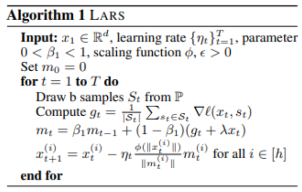
Figure 1. Pseudocode for LARS showing the hyperparameters used during HPO
| Hyperparameters for RN50 | Symbol | Type | Constraint |
|---|---|---|---|
| Number of Training Epochs | NTE | INT | Positive INT |
| Number of Warmup Epochs | NWE | INT | Positive INT |
| Base Learning Rate | BLR | FLOAT | Positive real |
| Weight Decay | WD | FLOAT | 0.0001 x 2N, N INT |
| Momentum | MM | FLOAT | Positive real, depends on global batch size |
Table 1. Hyperparameters and MLPerf constraints
Integration of Large-Scale Training and HPO Workflow Processes
Figure 2 shows a conceptual representation of the training cluster that could be on-premise or cloud-based. It is being accessed by an AI user who submits batches of training jobs to the computing infrastructure. The user gets back the accuracy on the runs (AC) and the number of converged epochs (CE). That information is fed to SigOpt, which responds back to the user with new hyperparameter suggestions. The user can program the criteria to continue, refine or stop the hyperparameter search once the optimization objective of finding the lowest possible convergence epoch while reaching the target accuracy is met.
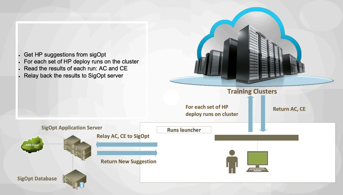
Figure 2. Running training jobs in the training clusters with SigOpt and the AI user controlling the HPO progress
HPO Workflow with SigOpt
Figure 3 illustrates our current HPO implementation of the workflow with SigOpt. SigOpt is started by defining the following variables:
- Initial boundaries of hyperparameters
- Threshold of evaluation metrics (e.g., AC)
- Experiment budgets (i.e., the number of runs we can afford within a time budget)
- Computational resources (i.e., the number of compute nodes to use)
- Parallel run budgets (i.e., the number of concurrent runs to speed-up the hyperparameter search within the allowed computational resources).

Figure 3. Workflow of HPO with SigOpt to find the HPs that meet target accuracy and minimize the number of epochs to converge.
The workflow consists of two nested loops with a set of building blocks with specific functionality: an inner loop (the dashed-dotted lines) and an outer loop (the dashed lines). After SigOpt is started, a new experiment is created and configured, and an evaluator algorithm is initialized with the hyperparameter boundaries. Then, the inner loop starts with suggested hyperparameter values provided by SigOpt, which uses the metrics from user training deep learning models on the training clusters to give recommendations. The inner loop completes its process once the predefined budget is reached.
Next, the outer loop starts by using the evaluator building block to validate the SigOpt hyperparameter suggestions and refines the boundaries based on user criteria. This allows you to bring your own additional optimizations on top of what SigOpt already provides. The evaluator we implemented leverages a K-means unsupervised machine learning clustering method, which will be described in the next section.
Once the hyperparameter boundaries are refined, the outer loop can resume its process for another iteration or stop when there is no improvement on the convergence epoch. The final suggestions of hyperparameter values are saved and the evaluation is stopped.
Bringing Your Own Evaluator into the HPO Workflow
Figures 4-7 illustrate the implementation of our evaluator, which is based on K-means clustering. For all data received from SigOpt, only the data meeting the accuracy requirement are saved, and these data are further filtered by keeping only 75% of the datapoints with the best converge epochs (Figure 4). Then, the K-means classification is applied to the suggested part of the datapoints (namely: NTE, BLR, NWE and WD) to separate them into clusters with each having at least ten datapoints (Figure 5). The cluster with the best performance is selected based on the minimum mean runtime (the blue dashed box in Figures 5 and 6).
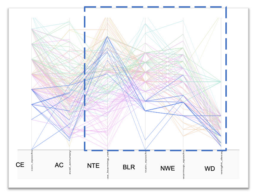
Figure 4. K-means clustering is applied to the parameter space of the measured points to group them into distinct clusters.
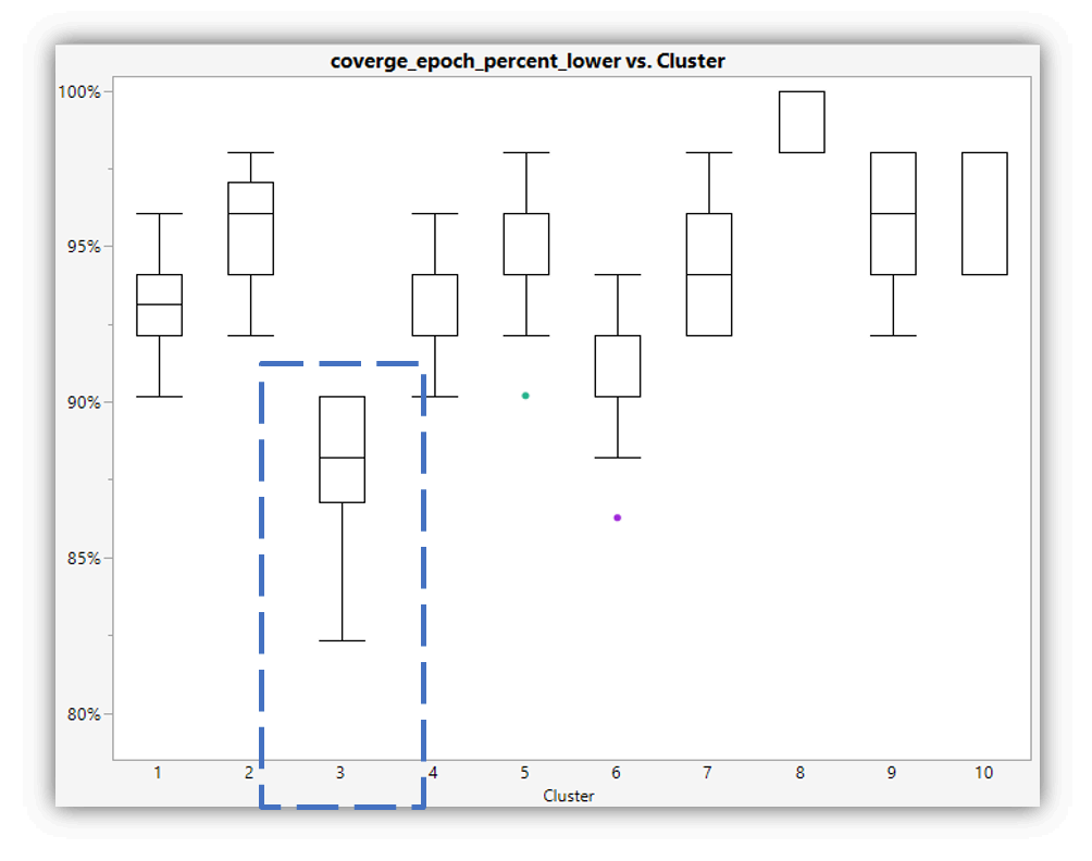
Figure 5. For each set of measurement in given cluster, the mean converge epoch is calculated. The blue square denotes the selected cluster with lowest mean converge epoch.
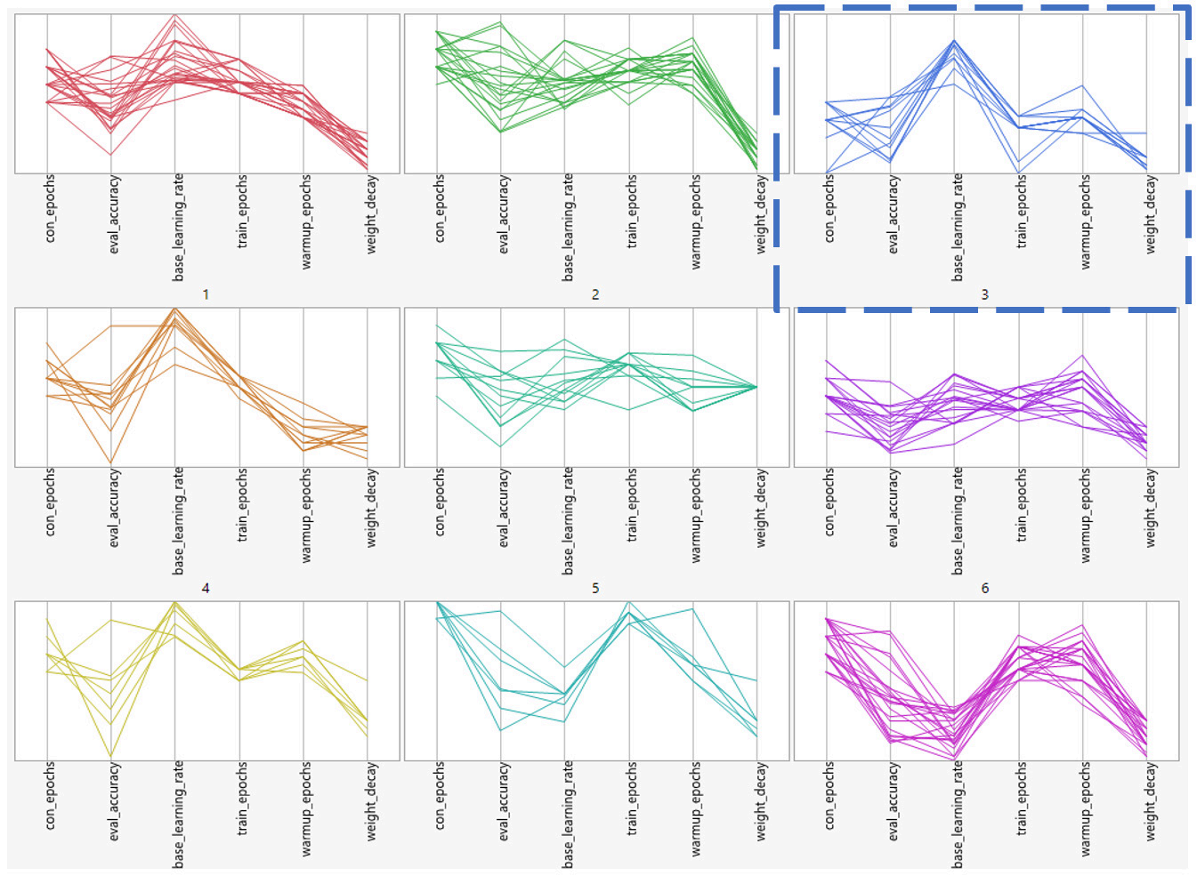
Figure 6. Measurement results clustered using the k-mean algorithm are plotted above. The selected cluster in Figure 5 is indicated by the blue square.
For a given hyperparameter, the range of values (boundaries) from the best cluster (with the lowest runtime/converged epochs) is compared with the SigOpt predefined boundaries (Figure 7). If any of the predefined boundaries (left and right in the range) are too close to any of the best cluster values found, the evaluator will adjust the corresponding SigOpt boundaries to allow the exploration of new hyperparameter values. On the other hand, if any of the SigOpt boundaries are far away from the best cluster values found, the evaluator will adjust the corresponding SigOpt boundaries to be closer to the best cluster hyperparameter value to allow for exploitation within the vicinity of that value. The 0.1 (10%) adjustment to the coefficient in Figure 7 is found empirically. We used 10% for RN50. The new adjusted SigOpt boundaries are then reconfigured for a new experiment. This adjustment speeds up the search of hyperparameter values. It is depicted graphically in Figure 8 for the learning rate hyperparameter. Due to the initial condition randomness of the deep learning framework, we executed each run several
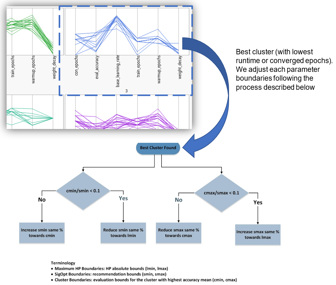
Figure 7. Illustration of the evaluator algorithm
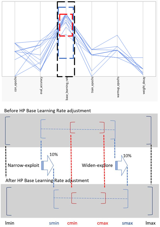
Figure 8. Hyperparameter value adjustment based on the best cluster hyperparameters
times with different random seeds for the parameter values. Then, we report the average and standard deviation for each metric to SigOpt. To speed up the search time and conserve compute resources we perform three runs for each data point during the search process. However, at end of the experiment we select the best set of points found by SigOpt and futher validate them with higher run counts (5-10 runs). This process will ensure that the results are stable and reproduceable. Running the optimization for a given global batch size also conserves compute resources because we are simultaneously covering a concurrent set of deployment senarios, each with different computing resources that share the same hyperparameters across different local batch sizes.
SigOpt Dashboard Charts
The charts embedded in the SigOpt dashboard such as parallel coordinates, contribution/sensitivity, and experiment history provide a set of complementary views that enrich the understanding of hyperparameters and their effects on convergence during an experiment. For RN50, we did 400 runs. The parallel coordinate plot (Figure 9) shows the relations between the hyperparameters suggested by SigOpt and the measured metrics (results) of these runs. The gray lines denote those runs that did not pass the target evaluation accuracy (SigOpt refers to it as the threshold), while the blue lines denote the runs that met the threshold. SigOpt highlights the best runs in orange (Figures 9 and 10). The parallel coordinate plots show correlations among the hyperparameters plus the accuracy and number of epochs to converge. For example, one can easily see that base_learning_rate and weight_decay are inversely correlated with the number of converged epochs.

Figure 9. RN50 parallel coordinate plot showing the relation between HPO and measured metric values

Figure 10. RN50 parallel coordinates for the best observations
Figure 11 shows the strong correlation between train_epochs and con_epochs. The con_epochs is simply the train_epochs number at which the target evaluation_accuracy is reached. As such, we expect a strong correlation. We can also see that con_epochs is approximately 1-3 epochs lower than train_epochs.
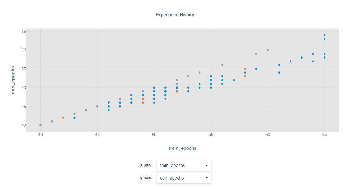
Figure 11. RN50 correlation between train_epochs and con_epochs
Figure 12 shows the contribution of each hyperparameter toward each of the metrics values. The orange and the blue bars show the contributions to eval_accuracy and con_epochs, respectively. The scale for the ranking is between 0 and 1 (100%). SigOpt uses the decision tree regressor model to measure these relations. In this figure, and as expected intuitively, we can see that train_epochs has the most impact on accuracy and con_epochs. Also, we can see that the weight decay parameter only impacts the con_epochs values, while base_learning_rate only impacts evaluation accuracy.
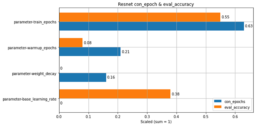
Figure 12. Relative contribution of the hyperparameter toward the metrics results for RN50. The scale is based on cumulative contribution of 100%.
Figure 13 is the main tracking plot in the SigOpt dashboard showing a scattered plot between all the metrics values. This plot updates during the experiment to show how the SigOpt optimizer is reducing con_epochs while improving evaluation accuracy. The best points are highlighted in orange. The best result is indicated by the red box.
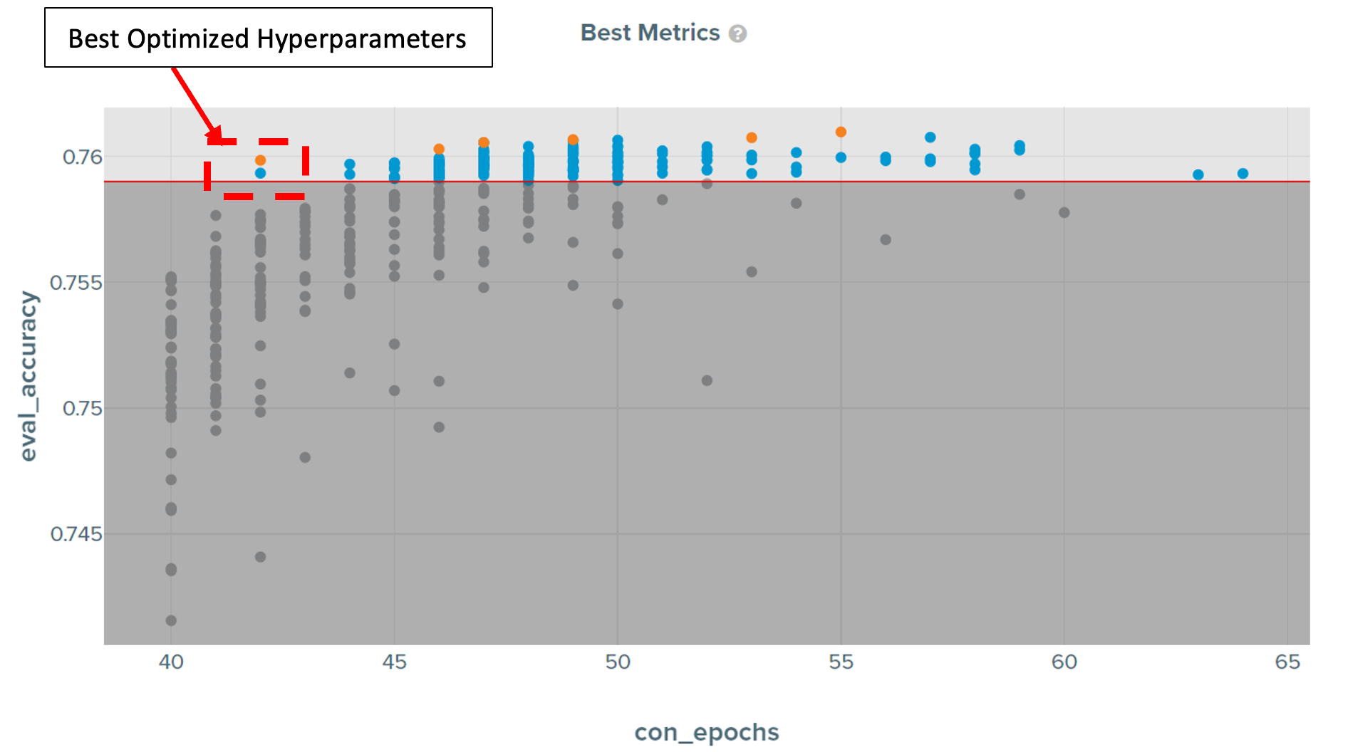
Figure 13. Correlation of best metrics
SigOpt HPO Results for MLPerf RN50
We start by providing the values used in HPO for both workloads. These are the hyperparameter values passed to MLPerf RN50 and the stopping criteria for the HPO workflow:
| Hyperparameter | Symbol | Type | Constraint |
|---|---|---|---|
| Number of Training Epochs | NTE | INT | 41 ~ 50 |
| Number of Warmup Epochs | NWE | INT | 2 ~ 15 |
| Base Learning Rate | BLR | FLOAT | 18 ~ 30 |
| Weight Decay | WD | FLOAT | 1.0e-5 ~ 4.0e-4 |
| Metric | Symbol | Type | Objective |
|---|---|---|---|
| Evaluation Accuracy | AC | FLOAT | > 0.759 |
| Converge Epoch | CE | INT | Minimize |
We close this section by listing the advantages of SigOpt over grid search found during MLPerf RN50 HPO:
- Found better hyperparameters with lower converge epochs (CE)
• Bayesian vs grid search
• 6% epoch reduction relative to grid search, which translates to ~6% lower training time - More efficient resource utilization
The following tables summarize the computational resources consumed during HPO and the runtime reduction achieved and expressed in terms of reduction of the convergence epochs.
| Cluster Runs | Grid Search Compute Resource Utilization (Hours) |
SigOpt Search Compute Resource Utilization (Hours) |
|---|---|---|
| K8s runs | 53,948 | 21,333 |
| Baremetal runs | 31,464 | 0 |
| Total runs | 85,413 | 21,333 |
| Grid Search | SigOpt Search | |
|---|---|---|
| Epoch reduction | 28% | +6% (in addition to grid search) |
Notice that the SigOpt search was performed after the grid search effectively starting from an already optimized search point. It was able to lower the converge epochs values by an additional 6% using less compute resources: 21,333 hours vs. 85,413 hours for SigOpt and Grid search, respectively.
Given these results, we hope AI developers will take advantage of the cost efficiency of Habana Gaudi and leverage SigOpt’s HPO to accelerate model development.