Neural networks are at the core of many modern-day artificial intelligence (AI) applications. The artificial neural network (ANN) is a model loosely based on the structure of a brain: It consists of connected elements called neurons, with each connection given a numerical weight. Convolutional neural networks (CNN) are special types of ANNs that can solve problems of computer vision (CV), such as image classification, object detection, and general recognition.
The major building blocks of CNNs are convolutional layers. These layers are made up of small filters that extract relevant features in images, with each layer extracting more abstract features based on the input from previous layers — all the way up to the final result. This approach works so well that state-of-the-art CNNs can outperform humans in accurately recognizing different people’s faces from a large set.
In this article, we’ll show you how to create a very simple CNN for image classification from scratch. We’ll use the following tools:
- Anaconda* Navigator to manage our project
- Intel® Distribution for Python* to develop base code
- Intel® Optimization for TensorFlow* to build and train our neural network
We’re assuming that you're familiar with Python and have a basic knowledge of neural networks to follow this guide.
You can install Intel distributions of the packages using these Anaconda commands:
conda install -c https://software.repos.intel.com/python/conda/ intelpython
conda install -c https://software.repos.intel.com/python/conda/ tensorflow
We recommend that you set up a deep learning (DL) environment with these tools on your working machine, as described in the article Building A Deep Learning Environment With Python And Anaconda.
Your First Neural Network
We’ll be using Python and TensorFlow to create a CNN that takes a small image of a typed digit from 0 to 9 and outputs what digit it is. This is a great use case to start with and will give you a good foundation for understanding key principles of the TensorFlow framework.
We’ll use the Intel Optimization for TensorFlow, which optimizes TensorFlow performance when running on Intel® architecture. The core of this optimization is the Intel® oneAPI Deep Neural Network Library (oneDNN), which is a set of building blocks for DL applications that includes convolutional and pooling layers — the base components of any CNN model. The library is a part of the Intel® oneAPI Base Toolkit, a set of libraries for developing high-performance AI, machine learning (ML), and other applications across diverse architectures.
The programming model of all oneAPI components is unified so that it can use the same code for deployment on CPU, GPU, or FPGA. Intel continues to develop oneAPI components to support new processors and optimize performance by taking advantage of new instruction set extensions.
Using oneDNN primitives as the back-end implementation for core TensorFlow algorithms provides higher performance for DNN models and ensures that the performance will be optimized for newer processor architectures.
Let’s Start Coding
Let’s get started with our simple CNN. This neural network classifies images with typed digits. The input for the network will be a small 28 × 28 pixel grayscale image, and the output will be an array of probabilities for each digit from 0 to 9. The first step is to build the TensorFlow model of the CNN. We’ll use the Keras API for this task, as it’s easier to understand when creating your first neural network.
Write and run the following code in your DL environment:
import os
os.environ['TF_ENABLE_ONEDNN_OPTS'] = '1'

import tensorflow
tensorflow.__version__
The first two lines of the code turn on the oneDNN optimizations for the session, and the last two lines check the version of the TensorFlow framework. Note that beginning with TensorFlow 2.9, the oneDNN optimizations are on by default and you have to set this to 0 if you wish to test performance without these optimizations.
Next, initialize the CNN model with the input layer:
from tensorflow.keras.models import Sequential
from tensorflow.keras.layers import Input

model = Sequential()
inp = Input(shape=(28, 28, 1))
model.add(inp)
We used the ‘Sequential’ model for our CNN. This model has the simplest structure with sequential layers where the output of one layer is the input of the next one. Then, we added the input layer to the model. All TensorFlow models need to know the type of input data. In our case, this is a tensor with three dimensions of 28, 28, and 1. This input corresponds to an image of 28 × 28 pixels with one color channel (a grayscale image).
The Convolutional Layer
Let’s continue and write the following code:
from tensorflow.keras.layers import Conv2D
conv = Conv2D(32, (5, 5), padding="same", strides=(1, 1))
model.add(conv)
The code initializes a convolutional layer ‘Conv2D’ and places it after the first input layer. This convolutional layer is the key element of our neural network. It’s in charge of extracting geometric features from input images, which are then used by the next layers. We created the layer with 32 kernels (or filters) of size (5, 5). The next two arguments specify how these filters are applied to the input image: strides specifies the vertical and horizontal shifts, and padding specifies whether the input image must be padded with extra pixels to process input data.
The Activation Layer
Any convolutional layer should be followed by an activation layer. This layer introduces an activation function to the model, which controls whether a neuron will “fire” (provide an output) based on its weight and its input. The most popular activation function for recent deep neural networks (DNN) is the rectified linear unit (ReLU). The following code adds the activation layer to our model:
from tensorflow.keras.layers import Activation
conv_act = Activation("relu")
model.add(conv_act)
The Pooling Layer
Another important element of a DNN is the pooling operation. The goal of the operation is to decrease the spatial dimension of the data that will be fed to the next layer. We’ll be using the max pooling operation, as it’s proven to be efficient in downsampling feature maps in CNN models.
from tensorflow.keras.layers import MaxPooling2D

pool = MaxPooling2D((4, 4))
model.add(pool)
The added MaxPooling2D layer was initialized with a pool size of (4, 4). This means the spatial dimension of the layer’s data output decreases by four times for both vertical and horizontal axes. So the initial 28 × 28 pixel image gets reduced to a 7 × 7 numeric output after the first layer, and so on.
The pooling operation has two purposes. One is to make the model independent of slight differences in extracted feature positions, and the other is to reduce the data amount for the next processing layers, thus making the model faster.
Visualizing Our Model So Far
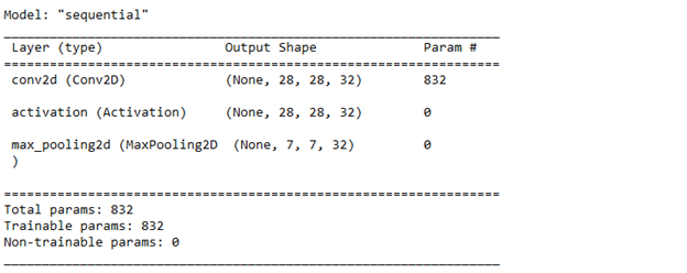
Now, our model consists of four layers: input, convolutional, activation, and pooling. At any stage of model building, we can view information on its structure by calling the model.summary method. The output of the method is shown in the image below:

We can see information about the output shape for every layer. For example, after the pooling layer, we can see that the spatial dimensions of the output decreased by four times from 28 to 7, just as expected. Another important piece of information is the number of trainable parameters in each layer. The convolutional layer in our model has 832 such parameters. Trainable parameters are coefficients (weights) of a layer, the values of which are tuned with the training process. The number of them directly affects the training time: the greater the number, the longer the training process.
The Flatten and Dense Layers
Let’s continue to build the model with the following code:
from tensorflow.keras.layers import Flatten
from tensorflow.keras.layers import Dense

flat = Flatten()
model.add(flat)

dense = Dense(128)
model.add(dense)

dense_act = Activation("sigmoid")
model.add(dense_act)
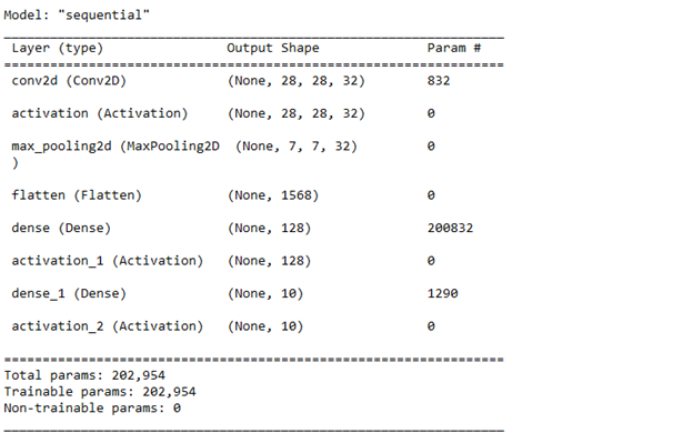
After this, our model outputs the following summary:

The code above adds a “flatten” layer that converts the three-dimensional tensor (7, 7, 32) from the pooling layer to a flat vector with 1568 components. It then adds a “dense” layer with 128 neurons and a sigmoid activation function to the model. This is the so-called hidden fully connected layer. It precedes the last classification layer, and its goal is to build a multilayer perceptron (MLP) in the last part of a neural model, as MLP is commonly the final block in classification neural networks.
The Classification Layer
The last layer of our model must be a classification layer with 10 output values: the probabilities for each digit. We’ll use a dense layer with 10 neurons and the Softmax activation function as a common choice for modern classifier models.
out = Dense(10)
model.add(out)

out_act = Activation("softmax")
model.add(out_act)
The final summary of our model is pictured below:

Training the Model
The next stage of model creation is loading the training and validation datasets. We’ll use a small dataset1 with 100 images for every digit in training data and 10 images in the validation one. Download the dataset and extract it to your working folder. We use the ImageDataGenerator class, which is a utility class that provides functions such as dataset loading, image preprocessing, and data augmentation. To load the datasets, run the following code right after the model creation:
from tensorflow.keras.preprocessing.image import ImageDataGenerator
datagen = ImageDataGenerator(rescale=1.0/255.0)

train_dataset = datagen.flow_from_directory("<your-train-data-file-path-here>", color_mode='grayscale', target_size=(28, 28), class_mode="categorical")
val_dataset = datagen.flow_from_directory("<your-validation-data-file-path-here>", color_mode='grayscale', target_size=(28, 28), class_mode="categorical")
This initializes the generator with the rescale parameter to normalize the image data to the interval of [0, 1.0]. When loading the data, we specified the class mode as categorical to generate the appropriate data for our classification problem.
The last step is to train our model using the datasets
from tensorflow.keras.optimizers import SGD

opt_method = SGD(learning_rate=0.1)
model.compile(optimizer=opt_method, loss="categorical_crossentropy", metrics=["accuracy"])

history = model.fit(train_dataset, validation_data=val_dataset, epochs=10)
We use the SGD optimizer, which should be the default choice when training a new model. The categorical_crossentropy is the recommended loss function for multi-class classification problems. The small count of 10 training epochs is enough for our simple model and small dataset. Here’s the output of the training process:

The final accuracy of the model is 96.6 percent for the training data and 94 percent for the validation data. Note that training the same model with the same data may produce slightly different results due to the nondeterministic nature of the process.
Testing It Out
Now we can test the model and run it for a single image:
from tensorflow.keras.preprocessing.image import load_img
from tensorflow.keras.preprocessing.image import img_to_array

img_file = "<your-test-data-file-path-here>\\7.png"
img = load_img(img_file, color_mode="grayscale")
img_array = img_to_array(img)
in_data = img_array.reshape((1, 28, 28, 1))/255.0

prob = model.predict(in_data)[0]
digit = prob.argmax()
digit_prob = prob[digit]

print(prob)
print("Predicted digit = " + str(digit))
print("Digit probability = " + str(digit_prob))
We get the following output:
[7.85533484e-05 1.45643018e-03 1.24442745e-02 1.29656109e-03
 1.41729815e-05 4.06741965e-05 4.37598487e-07 9.83559847e-01
 3.04310001e-04 8.04647047e-04]
Predicted digit = 7
Digit probability = 0.98355985
The model correctly predicted that the image contains the digit 7 with a good probability of about 98 percent.
Congratulations! You’ve created your first neural network. If you wish to save your trained model, you can use the following command:
model.save("<your-model-file-path-here>”)
Conclusion
In this article, we learned how to create a very simple neural network with the TensorFlow framework. As a practical example, we built a CNN for classifying images with typed digits. We provided the steps to build a sequential model with two blocks. The first block, containing a convolutional layer, acts as a feature extractor. The second block, a perceptron with one hidden fully connected layer, is a common classifier that’s often used in modern DNNs.
While training our model and running inference, we sped up turnaround times by using the Intel Optimization for TensorFlow. This version of the framework is powered by the oneDNN library, part of the oneAPI toolkit for AI applications.
Although we created a very simple neural network, this demonstrates how it is easy to build and train DNNs with the TensorFlow framework. Modern state-of-the-art models contain hundreds and even thousands of layers, and the TensorFlow framework allows you to create them easily while the Intel Optimization for TensorFlow speeds up training and inference runs.